Jimena
Jimena is a Java genetic regulatory network simulation framework which focuses on computational efficacy and a modularized architecture to facilitate the development and testing of new algorithms and models surrounding GRNs. It features
- Network import from yED graph files (Example 1: Download (source), Example 2: Download)
- Full support of the exponential interpolation model implemented in SQUAD
- Full support of the polynomial interpolation models implemented in Odefy, including a significantly better implementation of the interpolation algorithm
- Several discrete update schemes
- Perturbation support in all models
- Several algorithms for the search of steady stable states in all models (fully multithreaded)
- In development: Network stability analyses, etc.
It is developed by Stefan Karl (stefan[dot]karl[at]stud-mail[dot]uni-wuerzburg[dot]de) at the Department of Bioinformatics of the University of Würzburg and supervised by Thomas Dandekar (head of the department).
Network input format
Activating influences are modeled using the yED standard arrow tip, inhibiting influences using any other tip (e.g. a diamond). Boolean nodes are modeled using nodes with the captions AND, OR, NOT, &&, ||, !. Cf. the examples above.
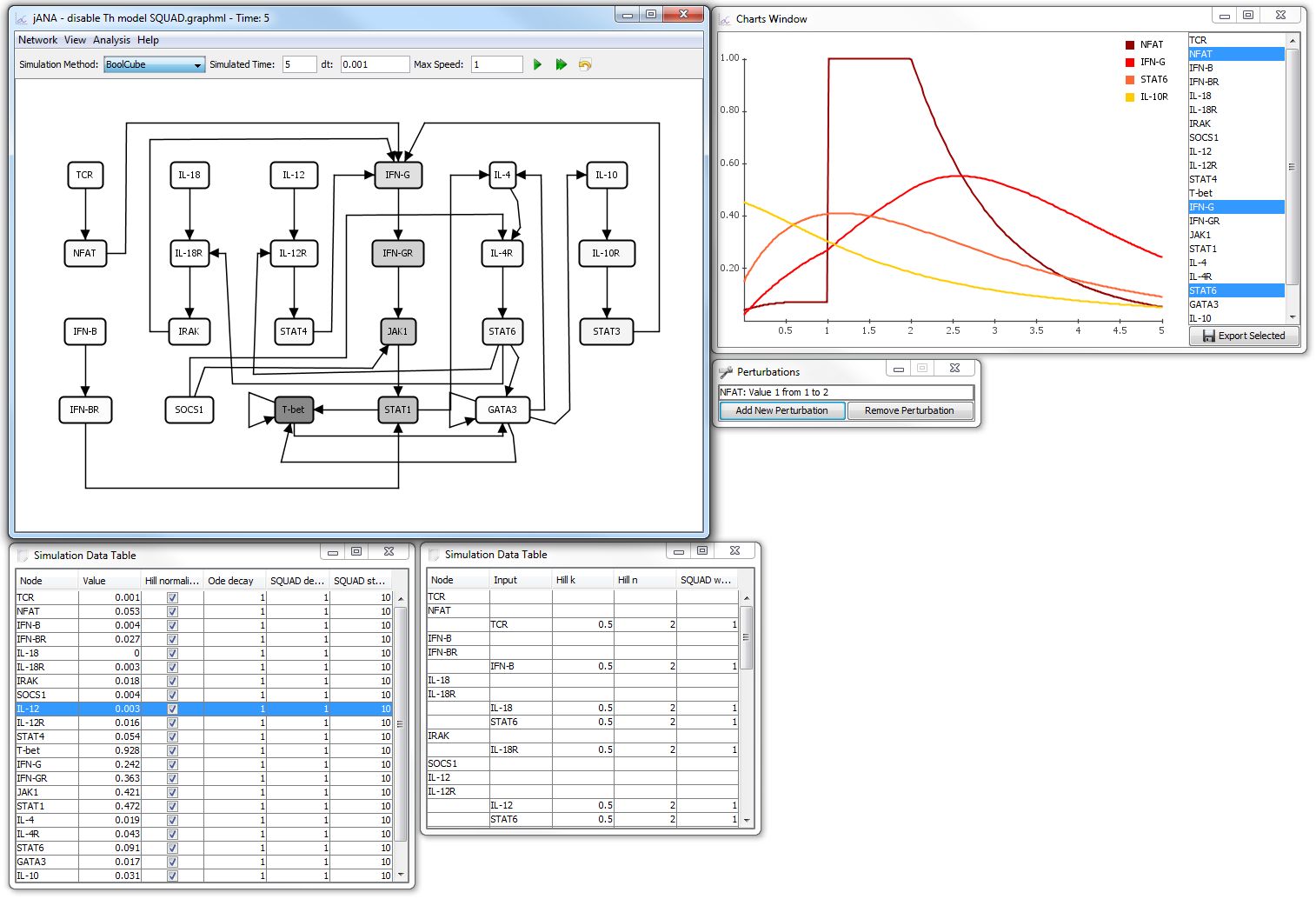
Screenshot
The screenshow shows a simulation of the T-helper network in the jIMENA GUI (which is not yet included in the release). The simulation was started from random values and the NFAT node was set to 1 between the time indices 1 and 2 by a perturbation.
Usage
The computational core of jIMENA is available as a jar-Library here (~0.4 MB, 22.03.2012). The GUI and and the source code will likely be released once all essential parts have been published.
You can easily make the library available to your project by adding it to your Java classpath (Eclipse: Right click on the Java-Projekt | "Properties" | "Java Build Path" | "Libraries" | "Add External JAR..." or create a library directory as shown here). It can then be used as demonstrated in this example.
You can also use the ready-to-use Eclipse workspace which contains the the example file and the library.
Download
Jimena is available as a zip file (current version, 26.02.2015), zip file (outdated version, Apr, 2014), zip file (outdated, ~0.6 MB, 16.09.2013). It runs both on windows (win xp, 7 and 8) and LINUX (ubuntu and suse are recommended). It can be used as a GUI application, for example by double-clicking on the jimena.jar file, or as a library in your java project. We recommend using the library version for a better control of simulations and analyses. The current source code ( zip file 12M, 22.09.2014, recommended) is also available.
The program and the source code are released under the GNU Lesser General Public License Version 3.
Jimena requires Java 7 or above.
Network can be edited with yed software (URL: https://www.yworks.com/products/yed/download).
You can easily make the library available to your project by adding it to your Java classpath (Eclipse: Right click on the Java-Projekt | "Properties" | "Java Build Path" | "Libraries" | "Add External JAR..." or create a library directory as shown here). Two example files are included in the zip archive.
We recommend reading the tutorial below which explains how to access Jimenas jar-file as a java library and how to use many of Jimena's essential funcions. A tutorial for the GUI is also available.
Graphml Converter
Jimena operates on .graphml files, such as those generated in the graph editor yEd.
However, networks often are stored in Tab delimited files that programs like R and Cytoscape can use as input.
To increase the compatibility of gramphl formats with other prorgams two parser in Perl language are provided.
"txt_to_graphm.pl" translates tab delimted files into graphml files and "2graphml_to_1graphml+txtout.pl" translates gramphl files into text files.
Contact
Prof. Thomas Dandekar
Dandekar group, Functional Genomics and Systems Biology department,
Lehrstuhl für Bioinformatik
Biocerter, University of Wuerzburg Am Hubland,
D-97074 Würzburg
Tel.: +49 (0)931 31 84551
Fax: +49 (0)931 31 84552
Ackowledgements
- JavaBDD (GNU LGPL) by John Whaley (http://javabdd.sourceforge.net) is used as a BDD framework.
- Icons (GNU LGPL) by Oxygen Team (http://www.iconarchive.com/artist/oxygen-icons.org.html)
- Several known GRN models have been implemented in Jimena. Cf. the papers for a comprehensive list.
- Support by DFG (Da 208/12-1) is gratefully acknowledged.
LIbrary tutorial
Using Jimena as a Java package
In this tutorial we assume that your Java IDE automatically adds import statements for classes you use in your code, as done by Eclipse. If this is not the case, please do it manually.
The network used in the examples is the Arabidopsis thaliana flower organ specification network version 2010. We suggest you follow the tutorial using the Example.java file which contains all of the code examples from below and some additional ones.
If you're using eclipse you could also open the ready-to-use workspace which already contains the library, an example network and the Example.java file.
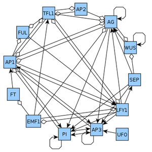
Figure 1: The Arabidopsis thaliana network used in the examples.
Step 1: Integrating the library into your Java project
To use Jimena as a library in your Java project, you have to add it to your build path. We lists the necessary steps for the frequently used IDE Eclipse. If you use another IDE please refer to its manual or the Java documentation.
- Start Eclipse and enter an Eclipse workspace.
- Create a new Java Project using File | New | Java Project. Enter a project name and click on Finish.
- The project appears in the Package Explorer. Right click on it and select Properties.
- Use Java Build Path | Libraries | Add External JAR... to add Jimena's jar file.
- Jimenas classes are now available in the project.
Step 2: Loading and configuring your network in Jimena
We can now load the network and set the values of the nodes and the parameters for the interactions.
- Create a yED graphml file containing your network. Activating influences are modeled using the yED standard arrow tip, inhibiting influences using any other tip (e.g. a diamond). Boolean nodes are modeled using nodes with the captions "AND", "OR", "NOT", "&&", "||" or "!" (examples). Parameters of the interactions such as the weight of an input, SQUAD's sigmoid gain etc. can be set after the network was loaded into Jimena.
- Create a new empty network using RegulatoryNetwork network = new RegulatoryNetwork();
- Load the yED network using network.loadYEdFile(new File("C:\\network.graphml")); where "C:\\network.graphml" is the path the your network.
- If necessary, you may now change the parameters of the interactions for the Odefy and/or SQUAD model. In the data structures of Jimena, the parameters are properties of the network nodes. You can access a network node via its index by using network.getNetworkNodes()[index] (for example in iterations) or via its name by using network.getNodeByName("AG"). In Jimena, SQUAD's γ parameter is called SQUADdecay (e.g. network.getNodeByName("AG").setSQUADDecay(2D);) and h is called SQUADsteepness. Odefy's τ equals OdefyDecay. Odefy's HillCube k and n parameters as well as SQUAD's αi and βi parameters are called HillKs, HillNs and SQUADWeights respectively. To find out which index in those arrays corresponds to which input node you may use the getInputIndicesByName function. For example, network.getInputIndicesByName("AG", "WUS") returns the indices of those inputs who originate from the node named "WUS" and lead to the node "AG". You could for example increase the influence of WUS on AG using
for (Integer index : network.getInputIndicesByName("AG", "WUS")){ network.getNodeByName("AG").getSQUADWeights()[index] = 2D; } - The value of a node can be set by using network.getNodeByName("FUL").setValue(1D);
Step 3: Simulating the network
After you have loaded the network and set the parameters for the interactions and the values of the nodes you can simulate the network from that state using several continuous and dicrete simulation methods:
network.simulate(new NormalizedHillCubeMethod(), 0.0001D, 10D, Double.POSITIVE_INFINITY,
1.0D, new BasicCalculationController());
- new NormalizedHillCubeMethod(): Specifies the simulation method. Other popular methodes include BooleCubeMethod, HillCubeMethod and NormalizedHillCubeMethod. For more examples refer to the classes in the package jimena.simulationmethods.
- 0.0001D: The step size of the diffential equation solver. 0.1 or 0.01 is enough in practice. (0.0001 is used here so that the calculation controller can be seen in action.)
- 10D: The network is simulated for 10 simulation time seconds/time units.
- Double.POSITIVE_INFINITY: The simulation is done as fast as possible. This parameter is used by the GUI to slow down the simulation so you can follow it as it is running. With a value of 2, for example, a maximum of two simulation time seconds are simulated in one real time second.
- 1.0D: Specifies that the state of the network is written into its log every 1.0 simulation time seconds. The log stores a history of the values of all nodes in the network.
- new BasicCalculationController(): A calculation controller outputs data on the current progress of the simulation. A BasicCalculationController writes the information to the standard output, a ProgressWindow opens a dialog window with the information and also allows you to abort the simulation. null is also possible.
After the simulation you can access the nodes to get their new values or the log to get a history of their values:
- System.out.println(network.getTimeIndex());: The network contains an internal time index which is 0 when the network is created or reset. After the simulation the time index has increased.
- System.out.println(network.getNodeByName("FUL").getValue());: Prints the value of the FUL node, which has changed after the simulation.
- The log of the network contains Point2D.Double values where the X-value is the time index of the log entry and the Y-value is the value of the node at that time:
for (Point2D.Double logEntry : network.getNodeByName("FUL").getLog()) { System.out.println(logEntry.getX() + ": " + logEntry.getY()); } - You can reset the network to reset all values to the initial values, reset the logs and set the time index to 0 using network.reset();. The simulation parameters and perturbations will not be affected.
Step 4: Perturbations
With perturbations you can assign one or multiple nodes a fixed or variable value (as a function of the time). This is especially useful to assign values to the input nodes (i.e. nodes without inputs) of the network and study the behavior of the network afterwards. Some basic perturbations can be found in jimena.perturbation, for example an OnOffPerturbation which assumes a constant value between two time indices start and end and is inactive otherwise. For example
network.getNodeByName("WUS").getPerturbations().add(new OnOffPerturbation(0, 100, 1));
sets the WUS node to 1 between t = 0 and t = 100. Perturbations can be deleted by directly accessing the list of perturbations (network.getNodeByName("WUS").getPerturbations().remove();) or deleting all perturbations at once (network.removeAllPerturbations();).
Step 5: Stable states
Jimena supports several steady stable state (SSS) searching methods. The most basic one, which is encapsulated in an RandomSearcher, is a randomly starting from points in the state space and simulating the network until a stable state is found. All methods also depend on the perturbations of the network, which for example allows for the calculation of SSS if the values of one or more nodes (e.g. input nodes) are fixed. The parameters are similiar to the simulation method:
network.stableSteadyStates(0.001D, 5D, new NormalizedHillCubeMethod(), 0.01D, 100D, 0.001D, 5000,
new ProgressWindow(), 4, new RandomSearcher());
- 0.001, 5: A state is considered stable if the the values of all nodes do not change by more than 0.001 during 5 seconds.
- new NormalizedHillCubeMethod(): Specifies the simulation method (see above).
- 0.01D: The step size of the diffential equation solver.
- 100D: The network is simulated for a maximum of 100 seconds. If no stable state is found until then, the simulation is aborted.
- 5000: SSS are searched for 5000 (real time) milliseconds.
- new ProgressWindow(): A progress window shows information about the calculation.
- 4: The calculation is distributed to 4 threads. Use as many threads as your CPU has (logical) cores (Runtime.getRuntime().availableProcessors()).
- new RandomSearcher(): A random sampling search method is used.
You can also search for just a single SSS starting from a given network state, in this example the current state of the network:
network.stableSteadyState(network.getValues(), 0.001D, 5D, new NormalizedHillCubeMethod(),
0.01D, 100D, new ProgressWindow());
The parameters are identical to the ones used in the previous example.
For discrete models (i.e. models in which the nodes can only assume a value of either 0 or 1) Jimena can determine all SSS with a simple method call:
network.discreteStableSteadyStates();